Plotting Output

Command line

Running the following from the command line will plot the variable significant wave height from the WAVEWATCH III at_4m grid. Note that the time of day (in this case, 15:00) is separated from the date with a T (i.e. times can be given as YYYY-MM-DDTHH)

ww3 plot --grid=at_4m --data-var=swh "2010-09-15T15"

Python

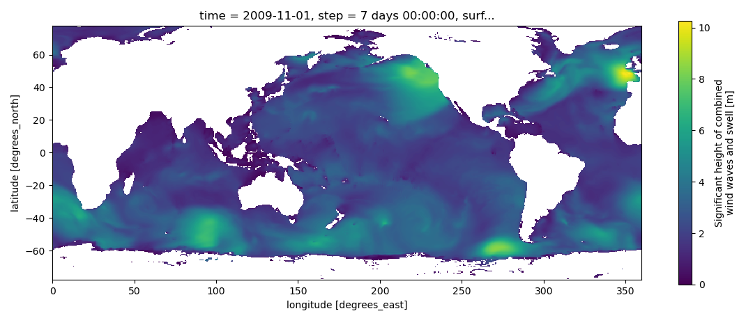
This example is similar to the previous but uses the bmi_wavewatch3 Python interface.

>>> from bmi_wavewatch3 import WaveWatch3
>>> ww3 = WaveWatch3("2009-11-08")

The data can be accessed as an xarray Dataset through the data attribute.

>>> ww3.data
<xarray.Dataset>
Dimensions:     (step: 241, latitude: 311, longitude: 720)
Coordinates:
    time        datetime64[ns] 2009-11-01
  * step        (step) timedelta64[ns] 0 days 00:00:00 ... 30 days 00:00:00
    surface     float64 1.0
  * latitude    (latitude) float64 77.5 77.0 76.5 76.0 ... -76.5 -77.0 -77.5
  * longitude   (longitude) float64 0.0 0.5 1.0 1.5 ... 358.0 358.5 359.0 359.5
    valid_time  (step) datetime64[ns] dask.array<chunksize=(241,), meta=np.ndarray>
Data variables:
    dirpw       (step, latitude, longitude) float32 dask.array<chunksize=(241, 311, 720), meta=np.ndarray>
    perpw       (step, latitude, longitude) float32 dask.array<chunksize=(241, 311, 720), meta=np.ndarray>
    swh         (step, latitude, longitude) float32 dask.array<chunksize=(241, 311, 720), meta=np.ndarray>
    u           (step, latitude, longitude) float32 dask.array<chunksize=(241, 311, 720), meta=np.ndarray>
    v           (step, latitude, longitude) float32 dask.array<chunksize=(241, 311, 720), meta=np.ndarray>
Attributes:
    GRIB_edition:            2
    GRIB_centre:             kwbc
    GRIB_centreDescription:  US National Weather Service - NCEP
    GRIB_subCentre:          0
    Conventions:             CF-1.7
    institution:             US National Weather Service - NCEP
    history:                 2022-06-08T16:08 GRIB to CDM+CF via cfgrib-0.9.1...

The step attribute points to the current time slice into the data (i.e number of three hour increments since the start of the month),

>>> ww3.step
56
>>> ww3.data.swh[ww3.step, :, :].plot()